The LogProduct
GRIB Files for Sailing: A Practical Passage-Planning Guide
Learn how to effectively use GRIB files for sailing to enhance your passage planning, improve safety, and monitor changing weather conditions.

Before your next departure, do this: request a targeted GRIB covering your route from NOAA/GFS via NOMADS or Saildocs, open it in a compatible viewer like XyGrib or OpenCPN, pull a second model for comparison, and plan conservatively wherever the two diverge. That single habit, comparing models rather than trusting one, is the most reliable safety signal GRIB files offer. When GFS and ECMWF agree on a weather window, your confidence is higher. When they show different wind directions or timing, treat that gap as a caution flag, not a coin flip.
Your immediate action list: choose a source (Saildocs for low bandwidth, NOMADS for direct download), define a tight bounding box around your route, request wind, gust, pressure, and wave fields at a 6-hour time increment, open the file in XyGrib or OpenCPN, and plan to update every 12–24 hours on passage.
Key Takeaways
GRIB files are most useful for sailing when you compare two models, match forecast time steps to your actual ETA at each waypoint, and treat divergence between models as a reason to delay or reroute.
| Point | Details |
|---|---|
| Request targeted GRIBs | Use Saildocs or NOMADS with a tight bounding box, 6-hour increments, and only the variables you need. |
| Compare two models | GFS and ECMWF agreement raises confidence; divergence of more than 12 hours or 10 knots means plan conservatively. |
| Watch resolution limits | GFS at ~18 miles (28 km) misses coastal effects; use higher-resolution data or local knowledge nearshore. |
| Monitor gust spread | A wide gust-to-mean gap signals atmospheric instability before pressure fields show it. |
| Update every 12–24 hours | A stale GRIB is worse than no GRIB; set a fixed update cadence and contingency thresholds before departure. |
Table of Contents
- What are GRIB files and why do sailors use them?
- Where can you get GRIB data for your passage?
- How do you request or download a fit-for-purpose GRIB?
- How do you open and view GRIB files on board?
- How do you read the key variables sailors actually need?
- How should you use model agreement to make passage decisions?
- What does a practical onboard GRIB workflow look like?
- Advanced tools for extracting and automating GRIB processing
- Why GRIB literacy still matters, even with better tools
- Sources
What are GRIB files and why do sailors use them?
GRIB stands for General Regularly-distributed Information in Binary form. It is the WMO-standard binary format for gridded meteorological data: compact, self-describing, and machine-independent. Every GRIB message carries its own metadata, including grid resolution, forecast time step, variable name, and units, so a viewer or script can decode it without a separate header file. That self-describing structure, combined with efficient binary compression, is exactly why GRIB became the format of choice for operational meteorology and why it transfers well over satellite or SSB radio.
GRIB1 vs. GRIB2 — what sailors need to know:
- GRIB1 is older, still common in some legacy services and older chartplotter plugins. Files typically use the
.grbextension. Precision is lower, and some longitude conventions differ from GRIB2. - GRIB2 is the current standard, used by ECMWF and modern GFS outputs. Files use
.grb2or.grib2. Higher precision, better compression, and wider variable support. Most modern viewers handle it natively. - Longitude quirks: some GRIB2 files encode longitude from 0° to 360° rather than the familiar -180° to 180°. Viewers that don’t account for this will render the Pacific basin oddly. Check your viewer’s settings if a file looks geographically shifted.
- Missing-value codes: GRIB files use sentinel values, often 9999, to flag grid points with no data. A viewer that misreads these as real values will show phantom wind speeds or wave heights. Always verify that your viewer handles missing-value flags correctly before relying on the output.
Where can you get GRIB data for your passage?
The right source depends on your mission, your bandwidth, and how much resolution you actually need.
| Source type | Cost | Best for | Bandwidth | Key features |
|---|---|---|---|---|
| Operational public models (NOAA/GFS via NOMADS, ECMWF open data) | Free | Offshore passages, global coverage | Moderate to high | Global models, direct download, multiple variables |
| Commercial multi-model services (PredictWind) | Paid subscription | Performance routing, offshore, multi-model comparison | Moderate | Proprietary models, route optimization, ensemble access |
| Email-request services (Saildocs) | Free | Low-bandwidth offshore, SSB/Iridium | Very low | Targeted GRIB by email, multiple model sources |
| Open-source mirrors and desktop services (OpenGribs/opengribs.org, zyGrib) | Free | Coastal and offshore desktop analysis | Low to moderate | Pre-configured downloads, desktop viewer integration |
Provider quick-reference:
- NOAA/GFS via NOMADS: The workhorse for global offshore planning. Free, updated four times daily, and accessible via direct HTTP download. Resolution is roughly 18 miles (28 km), which is adequate for open-ocean legs but coarse for coastal features.
- ECMWF: Widely regarded as the most accurate global model. The ECMWF open data portal provides some public access; full resolution data (roughly 5.6–11.2 miles / 9–18 km) is available through commercial redistribution partners. Worth the extra step for long offshore passages.
- Saildocs: Delivers GRIB files by email, making it the go-to for passages where you’re relying on SSB radio or a metered satellite connection. Supports GFS, ECMWF, and regional models.
- PredictWind: A commercial service offering its own proprietary models alongside GFS and ECMWF, with a built-in routing engine. Useful when you want multi-model comparison and route optimization in one interface.
- OpenGribs / opengribs.org and zyGrib: Open-source desktop tools that let you download and view GRIBs without a subscription. zyGrib is the older, well-established viewer; XyGrib is its actively maintained successor under the OpenGribs project.
For offshore passages, ensembles beat a single deterministic run. Ensemble products show the spread of possible outcomes across many model runs, giving you a direct read on forecast uncertainty rather than forcing you to compare two separate deterministic outputs manually.
How do you request or download a fit-for-purpose GRIB?
The goal is the smallest file that covers your route with enough resolution and time horizon to make a real decision. Here’s a repeatable workflow:
- Define your bounding box. Draw a rectangle around your route with a margin of roughly 100–200 nautical miles on each side. Tighter boxes mean smaller files and faster transfers.
- Choose your variables. For most passages: wind speed (10m U and V components), wind gusts, mean sea level pressure, significant wave height, and wave period. Rain and cloud cover are optional but useful for squall detection.
- Set your time window and increment. For a 5-day passage, request 120 hours. Use a 6-hour increment for planning; 3-hour if you’re in a fast-moving weather system. Longer increments cut file size significantly.
- Pick your resolution. For open-ocean legs, 0.5° (roughly 30 miles) is sufficient. For coastal passages with complex terrain, request 0.25° or finer if the source supports it.
- Request via Saildocs or direct download. For low-bandwidth connections, Saildocs is the most reliable option.
Saildocs email request example:
Send a plain-text email to [email protected] with a subject line like send GFS and a body like:
send GFS:30N,50N,10W,30W|0.5,0.5|0,6,12,...,120|WIND,PRMSL,WAVESBreaking that down: GFS is the model; 30N,50N,10W,30W is your bounding box (lat/lon); 0.5,0.5 is the grid spacing in degrees; 0,6,12,...,120 is the forecast time series in hours; and WIND,PRMSL,WAVES are the requested variables. Edit the bounding box and time series for your route, and Saildocs returns the GRIB file as an email attachment, typically within a few minutes.
Bandwidth pro-tips:
- Request only the variables you will actually use. Each additional field adds to file size.
- Prefer 6-hour increments over 3-hour when bandwidth is tight. You lose some temporal detail but cut file size roughly in half.
- On Iridium or SSB, a well-targeted GFS GRIB for a 5-day Atlantic crossing can stay under 50 KB.
- After download, verify: check the file extension (
.grbor.grb2), confirm the forecast reference time matches your expected update cycle, and open the file immediately to confirm it renders without errors.
How do you open and view GRIB files on board?
Your viewer choice depends on your platform and whether you need chart overlay, routing, or just raw field visualization.
- XyGrib (Windows / macOS / Linux): The actively maintained successor to zyGrib, free and open-source. Handles GRIB1 and GRIB2, displays wind barbs, pressure isobars, wave height, and rain. Clean interface, good for pre-departure desktop analysis.
- zyGrib (Windows / macOS / Linux): The predecessor to XyGrib, still functional and widely used. Slightly older interface but reliable for standard GFS and ECMWF downloads.
- OpenCPN (Windows / macOS / Linux / Android): The open-source chartplotter that most offshore sailors already have installed. Its weather plugin overlays GRIB wind, pressure, and wave fields directly on your chart, which is the closest thing to a chartplotter-native GRIB experience on a laptop or tablet.
- LuckGrib (macOS / iOS): A polished commercial viewer with excellent ECMWF and GFS support, ensemble visualization, and a clean mobile interface. Worth the cost if you’re on Apple hardware and want a refined experience.
- PredictWind viewer: Bundled with a PredictWind subscription, it offers multi-model overlay and route optimization. Strong for offshore passage planning when you want routing and GRIB visualization in one tool.
- Chartplotter plugins: Many modern chartplotters (Garmin, Raymarine, B&G) accept GRIB overlays via proprietary apps or SiriusXM/Iridium feeds. Compatibility varies by device and firmware version. Vendor-specific plugins often support only a subset of GRIB variables and may lag behind the latest GRIB2 spec, so verify before departure.
For quick inspection without a GUI, two command-line tools are worth knowing:
- wgrib2: Lists the inventory of a GRIB2 file, extracts specific messages, and converts to other formats. Useful for scripting and verifying file contents before opening in a viewer.
- ecCodes (ECMWF): Provides
grib_lsfor listing message metadata andgrib_dumpfor full message inspection. The NCEP reading guide covers wgrib/wgrib2 as standard inventory tools; ecCodes extends that to full programmatic decoding.
How do you read the key variables sailors actually need?
Wind, pressure, and waves are the three fields that drive passage decisions. Everything else is context.

Wind fields: GRIB files store wind as U (east-west) and V (north-south) component vectors at 10 meters above the surface. Viewers convert these to speed and direction and render them as wind barbs. One full barb = 10 knots; a half barb = 5 knots; a pennant = 50 knots. Wind speed is typically in meters per second in the raw file; good viewers convert to knots automatically. Always confirm the unit display setting before reading a chart.
Gust fields (usually labeled GUST or 10m wind gust) represent the peak 3-second wind within a forecast period. A large spread between mean wind and gust, say 15 knots mean with 28-knot gusts, signals a convective or unstable air mass. That gap is a volatility indicator worth watching as closely as the mean wind itself.
Model resolution and what it means for your interpretation:
| Model | Approximate resolution | Best use case |
|---|---|---|
| GFS (NOAA) | ~18 miles (28 km) | Open-ocean passages, global coverage |
| ECMWF | ~5.6–11.2 miles (9–18 km) | Offshore passages, higher accuracy |
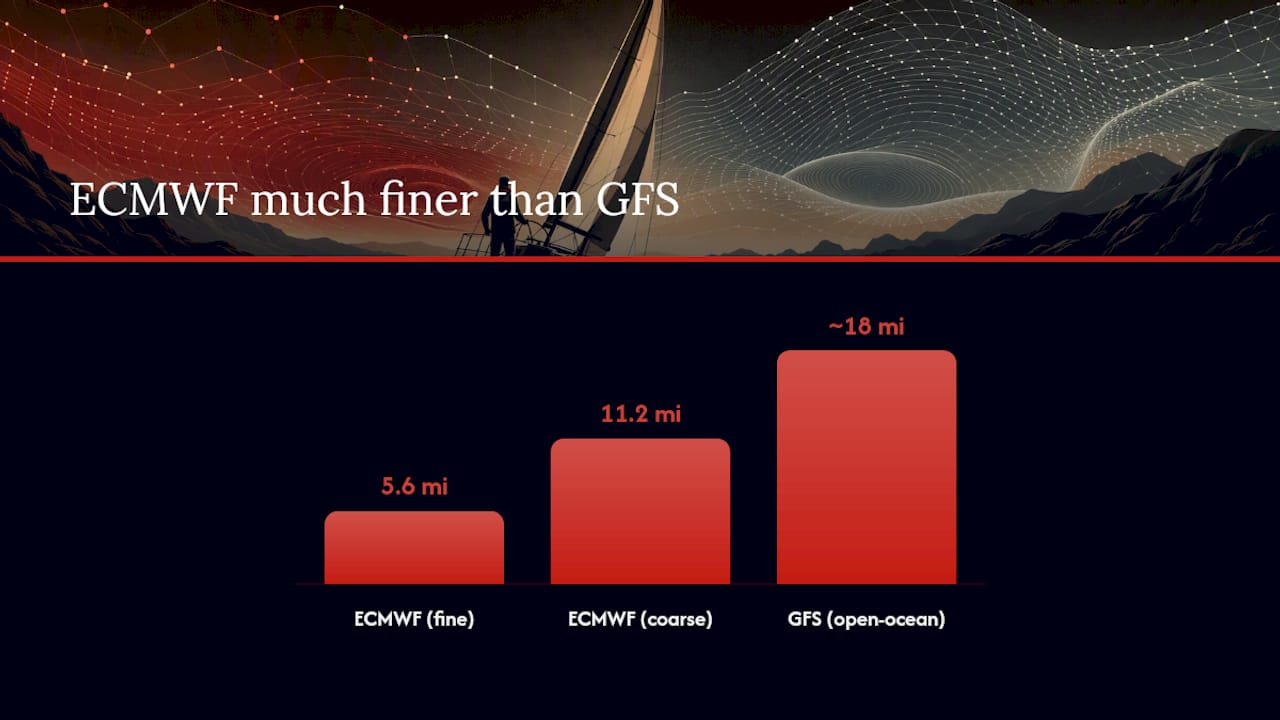
As Cruising World notes, a single GFS grid point at 18-mile spacing represents hundreds of square miles. Coastal wind acceleration around headlands, channel effects, and bay breezes simply don’t appear at that resolution. Use higher-resolution products or local knowledge to fill that gap nearshore.
Pressure fields: Isobars spaced tightly together mean a steep pressure gradient and stronger winds. A 4 mb drop over 60 miles is a very different situation from the same drop over 600 miles. Most viewers draw isobars automatically; watch for tightening between forecast steps as a sign of developing conditions.
Wave fields: Significant wave height (SWH) is the average of the highest one-third of waves, not the maximum. A 3-meter SWH means occasional waves of 4.5–5 meters are plausible. Wave period matters as much as height: a 12-second swell at 3 meters is far more manageable than a 6-second chop at the same height. Wave direction tells you whether swell and wind waves are aligned or crossing, which affects comfort and boat speed.
Pro Tip: Check the spread between mean wind and gust in every forecast step. A widening gust-to-mean ratio over your passage window often signals increasing atmospheric instability before the pressure field shows it clearly.
How should you use model agreement to make passage decisions?
A single GRIB forecast is a hypothesis. Two models that agree on that hypothesis make it a working plan. Two models that disagree make it a reason to wait.
The practical rules:
- When GFS and ECMWF agree on wind direction, timing, and magnitude within a reasonable margin, your confidence in that window is higher. Plan for it, but build in a buffer.
- When they diverge on timing by more than 12 hours or on wind strength by more than 10 knots, treat the more conservative scenario as your planning basis. Delay ETD if the divergence falls within your passage window.
- Ensemble spread is the cleaner signal. An ensemble with tight clustering around a forecast value means the atmosphere is in a predictable state. Wide spread means the models themselves are uncertain, and that uncertainty is real, not a modeling artifact.
- Regional model bias is real. Experienced navigators track which model performs better in their sailing region and season, then weight that model more heavily. GFS tends to underestimate trade-wind strength in some Atlantic corridors; ECMWF can be slow to resolve rapidly deepening lows. Build your own mental calibration over time.
- Update frequency matters. On a 5-day passage, pull a fresh GRIB every 12–24 hours. If a new run shifts the forecast significantly, reassess your route and contingency anchorages before the weather arrives.
The decision-rule framework is simple: agree = proceed with margin; diverge = wait or reroute; ensemble spread wide = treat the pessimistic scenario as real.
What does a practical onboard GRIB workflow look like?
A repeatable pre-departure and on-passage routine keeps GRIB use efficient and safe.
- Define bounding box and variables the evening before departure. Include your full route plus contingency ports.
- Request or download the GRIB via Saildocs (email) or direct download. Confirm file size and extension on receipt.
- Open and verify timestamps. Check that the forecast reference time is current (within the last 6 hours for GFS, 12 hours for ECMWF). A stale GRIB is worse than no GRIB.
- Compare two models or one deterministic plus one ensemble. Note where they agree and where they diverge. Mark divergence zones on your chart.
- Overlay your route on the viewer. Step through each forecast time to watch conditions evolve along your track, not just at the destination.
- Set your update cadence. Every 12 hours on passage is the practical minimum. Every 24 hours is acceptable in stable, high-confidence conditions.
- Define contingency thresholds before you leave. Decide in advance: if wind exceeds X knots or wave height exceeds Y meters at waypoint Z, you divert to the nearest shelter. Deciding this at anchor is far easier than deciding it at sea.
Pro Tip: When bandwidth is critically low, prioritize wind and pressure fields over waves and rain. Wind and pressure drive the go/no-go decision; wave fields are secondary context. A 10 KB wind-only GRIB beats no update at all.
Integrating GRIB overlays with your chartplotter route requires one caution: GRIB time steps and your ETA at each waypoint must align. A forecast showing 20 knots at a waypoint for the 06:00 step is irrelevant if you’ll arrive at 18:00. Step through the time series to match forecast conditions to your actual ETA at each point, not just the departure time.
Advanced tools for extracting and automating GRIB processing
For sailors who script their own weather pipelines or work with large GRIB archives, these tools are the standard stack.
- wgrib2: The most widely used CLI tool for GRIB2 inventory and extraction.
wgrib2 file.grb2lists all messages with variable names, levels, and forecast times.wgrib2 -match ":UGRD:10 m:" file.grb2 -csv output.csvextracts the 10-meter U-wind component to CSV. The NCEP reading guide covers wgrib/wgrib2 as the standard inventory approach. - ecCodes (ECMWF): The ECMWF ecCodes toolkit provides
grib_lsfor a quick message inventory,grib_dumpfor full message content, andgrib_get_datafor extracting grid-point values. Example:grib_ls -p shortName,level,stepRange file.grb2prints a clean summary of all messages. ecCodes handles both GRIB1 and GRIB2 and is the recommended toolkit for programmatic decoding. - cfgrib + xarray: cfgrib is a Python interface that opens GRIB files as xarray datasets using ecCodes under the hood. It supports lazy loading, so you don’t load the entire file into memory. On first open, cfgrib writes a
.idxindex file alongside the GRIB; subsequent opens use the index for fast access. Usefilter_by_keys={'shortName': 'u10'}to load only the variable you need. This is the right tool for automated passage-planning scripts or integrating GRIB data into routing calculations. - GDAL: The GDAL GRIB driver reads GRIB1 and GRIB2 as raster layers, enabling conversion to GeoTIFF or other formats for GIS workflows. GDAL supports external index files for faster selective access on large files hosted remotely, including S3-hosted archives. Watch for longitude wrapping issues when reprojecting GRIB data that uses 0°–360° longitude encoding.
Troubleshooting quick-reference:
- Mixed GRIB1/GRIB2 files in the same archive: use
grib_lsto identify edition numbers before processing. - Longitude wrap issues: check whether your file uses 0°–360° encoding and configure your tool accordingly.
- Slow opens on large files: generate a
.idxfile with cfgrib or use wgrib2’s index option to avoid full-file scans on every access.
Why GRIB literacy still matters, even with better tools
There’s a temptation to treat a polished weather app as a substitute for understanding what’s underneath it. It isn’t.
Every routing recommendation, every color-coded wind overlay, every “go/no-go” suggestion from any tool ultimately traces back to a GRIB file from GFS, ECMWF, or a regional model. When you know how to read that file directly, you can catch a stale forecast, spot a resolution artifact near a headland, or notice that two models are telling very different stories before the weather arrives. That’s not a technical skill for its own sake. It’s seamanship.
The passage that changed my thinking wasn’t dramatic. Two models disagreed by about 18 hours on the timing of a front crossing the Bay of Biscay. The app I was using showed a clean window. The raw GRIBs showed a disagreement I couldn’t ignore. We waited a day. The front came in 14 hours early. A GRIB file didn’t save us; reading two of them did.
Combine GRIB analysis with local observation, VHF weather broadcasts, and conservative seamanship. The file is a tool, not a guarantee.
Sources
- What are GRIB files and how can I read them - Copernicus Knowledge Base - ECMWF Confluence Wiki
- How to Read and Interpret GRIB Weather Files
- Saildocs

Raw GRIB analysis tells you what the atmosphere might do. Nausika connects that analysis to validated, real-time maritime data inside your existing AI assistant, adding live forecasts, routing context, and harbor information sourced from verified marine datasets. If you want to see how GRIB-derived forecasts integrate with an AI-powered maritime workflow, the Nausika roadmap shows what’s coming next for routing and forecast integration.