The LogProduct
Wave Breaking Depth: Formulas and Field Guide
Discover how to determine wave breaking depth with essential formulas and practical insights to enhance your coastal understanding.

A wave typically breaks when water depth reaches roughly 1.3 times the breaking wave height — so a 3-foot wave breaks near 3.9 feet of depth. Flip this around and you get the breaker index γ = H_b / h_b, which averages 0.78–0.88 across most shorefaces. The equivalent steepness limit, H/L ≈ 1/7 (Miche’s criterion), tells you when a wave is too steep to survive regardless of depth. And the depth-limited rule H ≈ 3/4·D (equivalently h_b ≈ 1.33·H_b) gives you a quick field check when you know only the local depth.
Worked example: Offshore significant wave height H₀ = 3 ft, peak period T_p = 8 s. Using the 1.3×H rule: h_b ≈ 1.3 × 3 ft = 3.9 ft. That is the depth at which you’d expect breaking to begin. Shoaling calculations confirm/03%3A_Voyage_III_Ocean_Physics/13%3A_Ocean_Waves/13.14%3A_The_Making_of_Surf) this order-of-magnitude estimate for a gently sloping shoreface.
Three caveats before you trust that number. First, bottom slope matters: a steep shoreface pushes γ above 1.0, so the wave breaks in deeper water than the rule predicts. Second, irregular ocean waves (spectral seas) break at lower average γ than monochromatic lab waves. Third, tidal stage shifts the absolute depth by feet or meters, moving the breakpoint shoreward on a falling tide and seaward on a rising one.
Key Takeaways
The most reliable first estimate for wave breaking depth is h_b ≈ H_b / 0.78, validated against the Miche steepness check and adjusted for tide and bottom slope before any operational decision.
| Point | Details |
|---|---|
| Core breaking-depth rule | h_b ≈ 1.3 × H_b (γ ≈ 0.78); a 3-ft wave breaks near 3.9 ft of depth. |
| Breaker index range | γ spans 0.6–1.2 depending on breaker type; spilling ≈ 0.6–0.8, plunging ≈ 0.8–1.2. |
| Slope and tide shift the breakpoint | Steeper slopes raise γ; a 6-ft tidal range can move the breakpoint by tens of meters on a 1:50 slope. |
| Irregular waves need adjusted γ | Spectral models like SWAN use lower effective γ (roughly 0.4–0.6) for irregular wave fields. |
| Nausika for operational use | Nausika integrates live buoy data, tidal levels, and marine forecasts to replace static-formula assumptions with current conditions. |
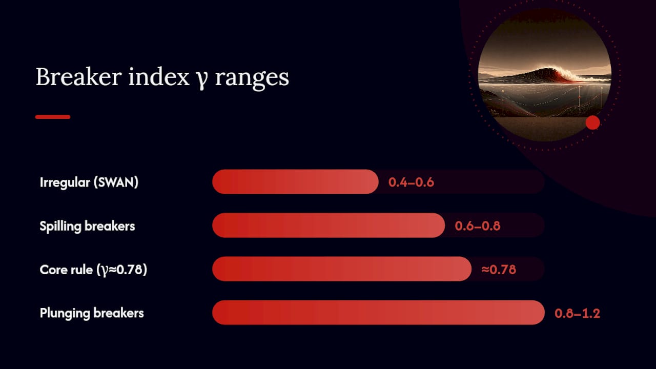
Table of Contents
- Why do waves break? Physics of shoaling and depth regimes
- What formulas do engineers actually use for breaking depth?
- How does bottom slope control breaker type?
- How to estimate wave breaking depth step by step
- Where breaking-depth estimates are used, and where they fail
- Why real-time validated data beats static rules for operational decisions
- Balancing rules-of-thumb and real data for safe decisions
- Nausika brings validated marine data to your breaking-depth workflow
- Sources
Why do waves break? Physics of shoaling and depth regimes
Ocean waves travel as oscillating pressure fields, and the water particles beneath them trace circular orbits in deep water. Those orbits shrink with depth, reaching negligible size at roughly half a wavelength below the surface. That boundary, D ≈ 1/2 L, is where a wave first “feels bottom” and begins to change character.
As a wave crosses into shallower water, its circular particle orbits flatten into ellipses. Horizontal velocities grow while the wave slows and shortens. When horizontal particle speed near the crest approaches the wave’s own celerity, the crest can no longer sustain itself — and it breaks. This is the physical core of the Miche criterion, and it produces the limiting steepness H/L ≈ 1/7 and the crest angle of roughly 120°.
Three depth regimes govern this progression:
- Deep water (D > 1/2 L): wave speed depends only on period; orbital motion is circular; no shoaling.
- Transitional water (1/20 L < D < 1/2 L): wave feels the bottom; wavelength shortens; height begins to increase (shoaling coefficient K_s > 1).
- Shallow water (D < 1/20 L): wave speed depends on depth alone (c = √(gD)); orbital motion is nearly horizontal; breaking is imminent.
The University of Hawaiʻi’s wave energy resource summarizes this progression clearly: waves feel bottom near D/L ≈ 0.5 and shoaling shortens wavelength while increasing height until instability triggers breaking. A useful mental image: picture the orbital circles gradually squashing into pancakes as the seafloor rises to meet them, until the top of the pancake outruns the wave itself.
The empirical criteria H/L ≈ 1/7 and H ≈ 3/4·D are not arbitrary — they follow from Stokes-wave theory and solitary wave solutions, respectively, and UBC’s sailing meteorology course treats them as the two practical limits taught to oceanography students: one for steepness-induced breaking (any depth), one for depth-induced breaking (shallow water).
What formulas do engineers actually use for breaking depth?
The breaker index γ
The breaker index is defined as:
γ = H_b / h_b
where H_b is the breaking wave height and h_b is the local water depth at breaking. Laboratory and field data place γ in the range 0.6–1.2, with most shorefaces clustering near 0.78–0.88. The inverse, h_b = H_b / γ, is the direct formula for wave breaking depth given a known or estimated H_b.
Miche’s steepness criterion
Miche (1951) derived a maximum steepness for a wave of any depth:
H/L ≈ 1/7 ≈ 0.142
In shallow water this reduces to the depth-limited form. In deep or transitional water it catches waves that are steep enough to break before they reach the shoreface — wind-driven whitecaps are a common example.
The depth-limited rule (H ≈ 3/4·D)
For shallow-water breaking, the solitary-wave approximation gives:
H_b ≈ 0.78 · h_b (equivalently h_b ≈ 1.28·H_b)
Many textbooks round this to H ≈ 3/4·D (γ = 0.75) for quick field use. The difference between 0.75 and 0.78 is smaller than the uncertainty from not knowing the exact bottom slope.
Goda’s and Battjes–Janssen adaptations
Goda’s formulation modifies γ to depend on both offshore wave steepness S₀ = H₀/L₀ and beach slope β. Steeper offshore waves and gentler slopes both reduce γ, while steep shorefaces increase it. Battjes and Janssen (1978) embedded a similar parameterization into a spectral energy-dissipation model, which became the backbone of the SWAN (Simulating WAves Nearshore) breaking module. A 2022 peer-reviewed study by Z. Chen proposes modified breaker-index formulas specifically for spectral wave models, noting that laboratory-derived γ values often need adjustment when applied to irregular wave fields in operational models.
Key points on applicability:
- Use the simple depth-limited rule for a first estimate on a gently sloping beach with regular swell.
- Apply Miche’s criterion when you suspect steepness-induced breaking before the wave reaches shallow water.
- Use Goda’s correction when you have a measured or estimated beach slope and offshore steepness.
- Use SWAN with a calibrated γ for irregular wave fields, harbor design, or any situation where the energy spectrum matters.
How does bottom slope control breaker type?
Bottom slope is the single biggest variable that the simple breaker-index formula cannot fully capture. It controls not just when a wave breaks but how — and the how has real consequences for surf quality, nearshore currents, and safety.
Spilling breakers
On very gentle slopes (roughly 1:100 or flatter), waves break gradually. The crest spills forward as a foamy, turbulent mass, dissipating energy over a long distance. Surfers know these as mushy, forgiving waves. γ for spilling breakers typically falls in the range 0.6–0.8. The gradual energy release means less intense nearshore currents but a wider surf zone.

Plunging breakers
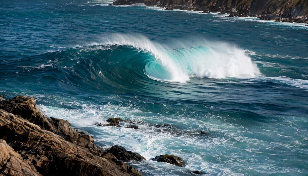
Moderate to steep slopes (roughly 1:20 to 1:10) produce the classic barrel wave. The crest pitches forward and curls over, trapping air before impact. Energy dissipation is concentrated and violent. γ rises to 0.8–1.2 for plunging breakers — meaning the wave can be taller relative to the depth at breaking than the simple 3/4·D rule suggests. Rip currents are strongest here, and the impact forces on coastal structures are highest.
Surging breakers
On very steep shorefaces or near vertical walls (slope > 1:8 or so), waves surge up the face without fully breaking. Most energy reflects back offshore. γ can exceed 1.0, and the wave breaking depth concept becomes less meaningful because the wave doesn’t dissipate in the conventional sense.
The UBC breaking waves resource confirms this slope-to-type mapping: gentle slopes favor spilling, moderate-steep slopes produce plunging, and very steep shorefaces produce surging. Field and flume evidence also show that γ decreases with larger offshore steepness and increases with steeper seabed slope, a dependence the Coastal Wiki breaker index entry documents in detail.
Pro Tip: If you’re assessing a new shoreface for the first time, estimate the Iribarren number ξ = tan(β) / √(H₀/L₀). Values below 0.4 indicate spilling, 0.4–2.0 plunging, and above 2.0 surging. This gives you a breaker-type prediction before you even enter the water.
How to estimate wave breaking depth step by step
You need four inputs: offshore significant wave height H₀ (or H_s), peak period T_p, a bathymetric profile or at minimum a single depth estimate at the location of interest, and the current tide level.
Step-by-step workflow
-
Compute deep-water wavelength. L₀ = (g · T_p²) / (2π). For T_p = 8 s: L₀ = (9.81 × 64) / 6.283 ≈ 99.9 m (≈ 328 ft).
-
Check depth regime. If your target depth D > L₀/2 (≈ 50 m here), the wave is still in deep water and won’t break there. If D < L₀/20 (≈ 5 m here), you’re in shallow water and depth-limited breaking applies directly.
-
Apply the Miche steepness check. Compute H₀/L₀. For H₀ = 3 ft (0.91 m) and L₀ = 99.9 m: H₀/L₀ ≈ 0.009. The limit is 1/7 ≈ 0.143. This wave is far below the steepness limit, so it won’t break in deep water — it will break when depth-limited.
-
Estimate breaking depth using the breaker index. h_b = H_b / γ. Assuming H_b ≈ H₀ for a gently shoaling beach (a conservative first pass), and γ = 0.78: h_b = 0.91 / 0.78 ≈ 1.17 m (≈ 3.8 ft). Using the simpler 1.3×H rule: h_b ≈ 1.3 × 0.91 m ≈ 1.18 m (≈ 3.9 ft). Both methods agree closely here.
-
Apply Goda’s correction if you know the slope. For a 1:50 beach slope and S₀ = 0.009, Goda’s formula reduces γ slightly below 0.78, pushing h_b a few centimeters deeper. For engineering design, this step matters; for a quick field check, step 4 is sufficient.
-
Adjust for tide. If the tide is 1.5 ft above MLLW at the time of interest, add 1.5 ft to h_b to get the absolute depth at breaking relative to the seafloor. The breakpoint moves seaward on a rising tide.
-
Iterate for irregular waves. For spectral seas, use H_s in place of H₀ and consider reducing γ to 0.5–0.6 for SWAN-type model inputs. The Chen (2022) modified breaker-index study provides updated formulas for this step.
Where to get your input data
- Wave height and period: NOAA NDBC wave buoys report H_s and T_p in near real time. Select the buoy nearest your area of interest.
- Bathymetry: NOAA’s Electronic Navigational Charts (ENCs) and the NOAA Coastal Relief Model provide gridded depth data. For precision work, use ADCP surveys or echosounder transects.
- Tidal predictions: NOAA Tides and Currents (tidesandcurrents.noaa.gov) provides station-based predictions and real-time water levels.
Pro Tip: Always run the Miche steepness check (step 3) before assuming depth-limited breaking. Storm waves with short periods can be steep enough to break in transitional water, well before reaching the shoreface — a fact that catches many first-time estimators off guard.
Where breaking-depth estimates are used, and where they fail
Applications
Coastal engineers use wave breaking depth to set the seaward boundary of surf-zone energy dissipation, which feeds directly into beach erosion models, breakwater design loads, and dredge-cut stability assessments. Harbor planners need to know whether incoming swell will break before reaching a channel entrance or remain unbroken and energetic inside a basin. Surf forecasters use breaker-index estimates to predict where and how powerfully waves will break at a given spot on a given tide. Search-and-rescue coordinators use breaking-zone maps to assess hazard areas for swimmers and small craft.
Limitations you can’t ignore
Simple formulas assume a uniform, planar shoreface. Real coastlines don’t cooperate. Sandbars shift the breakpoint shoreward by tens to hundreds of meters compared to a smooth-bottom prediction. Bar-trough systems create multiple breaking zones, each with its own γ. Fine-scale bathymetric features — a submerged rock, a channel edge — can trigger breaking in water far deeper than any formula predicts.
Wave direction matters too. When swell approaches obliquely, refraction concentrates energy on headlands and shallow points, which break first. The breaker then propagates alongshore, creating hazard patterns that a single-point depth estimate completely misses. This is the wave direction spread problem: a formula gives you one number, but the real breakpoint is a zone with spatial structure driven by approach angle.
Tidal variability compounds everything. A 6-foot tidal range shifts the breakpoint by tens of meters on a 1:50 slope. An estimate made at high water can be off by the full tidal range at low water.
Pro Tip: *For any high-consequence decision — harbor entry in swell, nearshore construction, rescue operations — compare at least three independent estimates: the Miche steepness check, the breaker-index depth-limited formula, and a live NOAA NDBC buoy observation.
Why real-time validated data beats static rules for operational decisions
A static rule-of-thumb workflow looks like this: you take H₀ from a forecast model, apply γ = 0.78, and get h_b. It takes 30 seconds and it’s often good enough for a rough check. But it carries hidden assumptions — that the bathymetry hasn’t changed since the last survey, that the tide is at a known stage, that the wave field is approximately monochromatic, and that the approach angle is normal to the shoreface. Any one of those assumptions can be wrong by enough to matter.
A data-driven workflow replaces each assumption with a measurement or a validated model output. Live NOAA NDBC buoy records give you H_s and T_p at the time of interest, not a 12-hour-old forecast. Up-to-date bathymetry from a recent survey or a high-resolution coastal model accounts for seasonal sandbar migration. A tidal prediction from NOAA Tides and Currents gives you the actual water level, not a mean. And a spectral wave model like SWAN, run with a calibrated γ, propagates the full energy spectrum through the bathymetry rather than treating the wave as a single height and period.
| Approach | Strengths | Primary failure modes |
|---|---|---|
| Static rule-of-thumb (γ = 0.78, H ≈ 3/4·D) | Fast, no data needed, good for first estimates | Ignores slope, tides, wave direction, bathymetric complexity |
| Goda/Miche with measured inputs | Accounts for slope and steepness | Still assumes regular waves, static bathymetry |
| SWAN spectral model with calibrated γ | Handles irregular seas, refraction, dissipation | Requires bathymetric grid, calibration data, computational resources |
| Real-time validated data (buoy + model + tide) | Captures current conditions, reduces assumption errors | Requires data access and integration workflow |
Coastal engineers describe the surf zone as an energy-dissipating system, and the Coastal Wiki recommends validating empirical breaker-index formulas against local observations and models rather than treating them as fixed constants. For shallow shorefaces, enclosed harbors, and high-consequence navigation, that validation step isn’t optional — it’s the difference between a safe passage and a grounding.
Nausika integrates validated real-time buoy records, live marine forecasts, and tide-aware depth data directly into AI assistant workflows, giving operational users the data layer that static formulas can’t provide.
Balancing rules-of-thumb and real data for safe decisions
Simple formulas are genuinely useful. A 30-second breaker-index calculation can tell you whether a wave is likely to break at a channel entrance before you commit to an approach. That’s real value, and dismissing it in favor of “always use a model” is impractical for most sailors and field engineers.
The honest guideline is this: use rules-of-thumb for orientation, and escalate to validated live data whenever the consequence of being wrong exceeds the cost of getting better information. A recreational surfer checking a new beach can use H ≈ 3/4·D and be fine. A harbor pilot navigating a swell-exposed entrance in a loaded vessel cannot afford that uncertainty. The threshold for escalation isn’t a formula — it’s a judgment about stakes.
Nausika brings validated marine data to your breaking-depth workflow
Static formulas tell you what should happen. Nausika tells you what the water is actually doing right now.
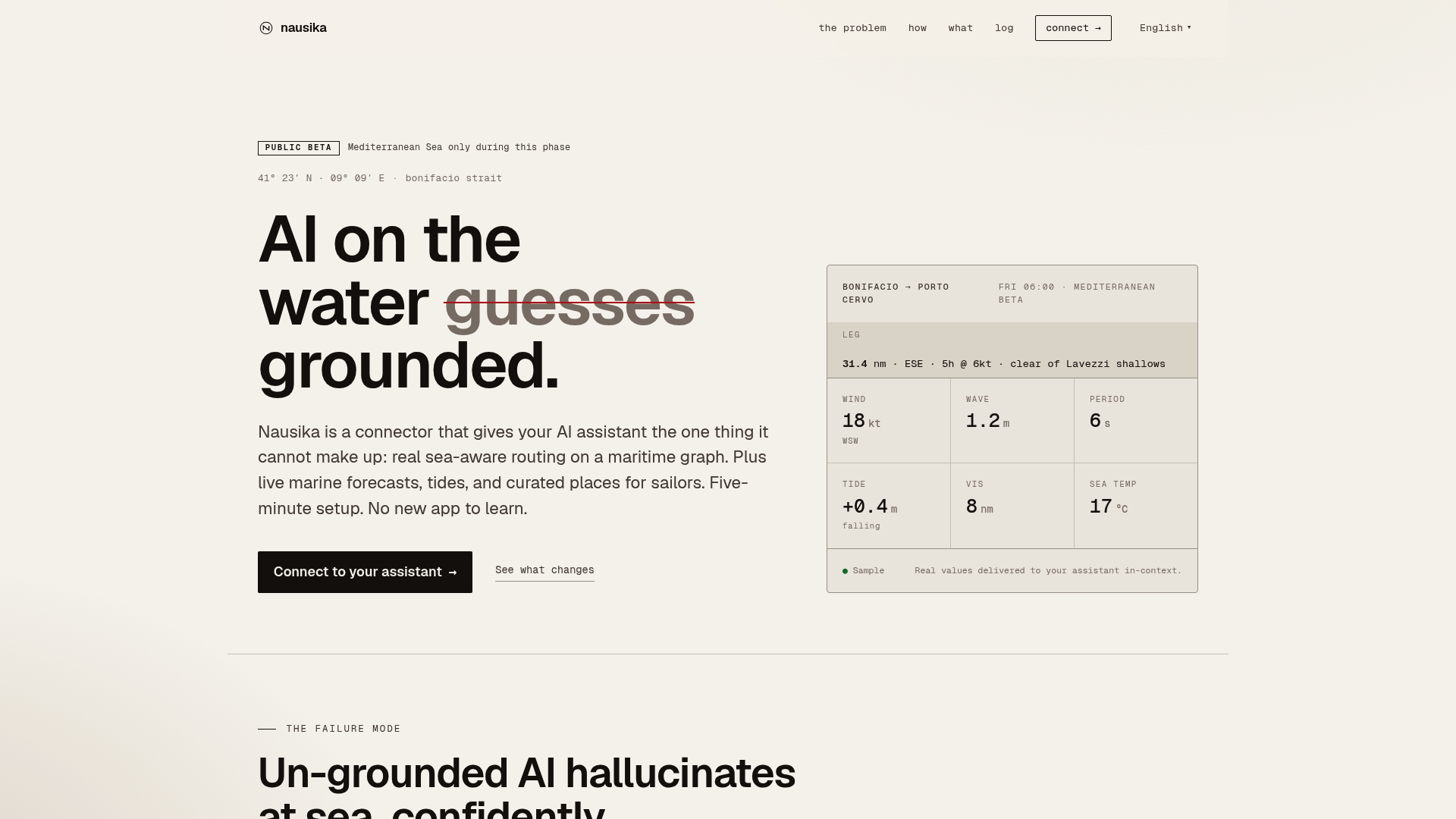
For sailors, charter operators, and marine professionals who need breaking-depth estimates that account for live conditions, Nausika connects validated buoy observations, real-time tidal data, and marine forecast outputs directly into your existing AI assistant. No new app. No manual data-hunting across NOAA pages. The inputs that matter — current H_s, T_p, tide stage, and local depth — are surfaced where you’re already working.
Nausika supplements engineering judgment and established models; it is not a replacement for professional structural design review or certified coastal engineering analysis. Think of it as the data layer that closes the gap between a textbook formula and the conditions outside your hull right now. See how Nausika integrates validated marine data into operational workflows, or visit Nausika to learn more and get started.
Sources
- Breaker index - Coastal Wiki
- Breaking waves - University of British Columbia (ATSC113 sailing meteorology)
- A modified breaker index formula for depth-induced wave breaking in spectral wave models - Z Chen (2022)